Tutorial 1: Generating the Basis and Worst-Case Paths

In this tutorial, you will explore how to use the sandbox script to generate the test cases that correspond to the basis paths of exemplar code. You will then use pre-obtained measurements of these test cases to generate other test cases that correspond to the five worst-case paths (or the paths with the longest predicted timings).

1. Run the executable gametime-cli located in the root directory of the GameTime distribution. This launches a command-line interface to GameTime: a window that contains a Cygwin prompt. Navigate to the root directory of the GameTime distribution.

2. The GameTime distribution includes several sample projects within the demo/sandbox directory. Copy the directory labeled modexp_unrolled, which constitutes the GameTime project for this tutorial, to the sandbox directory: cp -r demo/sandbox/modexp_unrolled sandbox

3. Examine the contents of the copied directory:

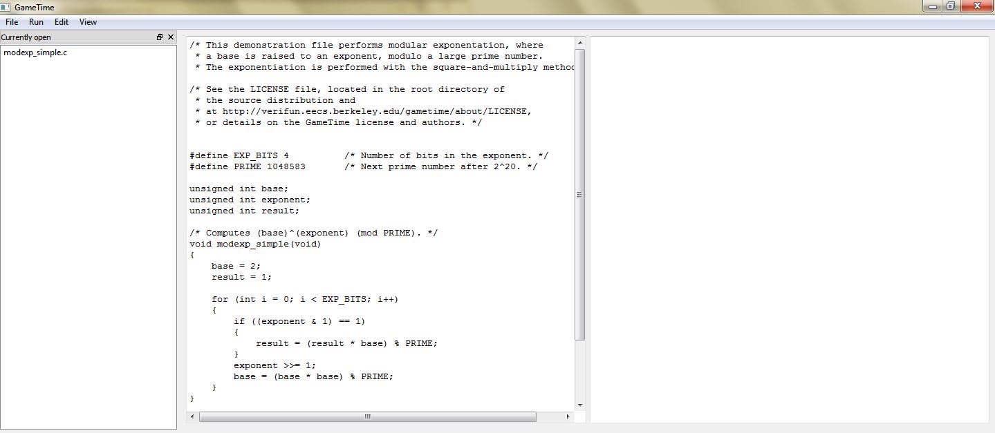
   • The C file, modexp_simple.c, contains an implementation of modular exponentiation, where a base (the global variable base) is raised to an exponent (the global variable exponent), modulo a large prime number. The code that will be analyzed is present in a function called modexp_simple.

     The function implements the square-and-multiply algorithm, with one conditional statement for each bit of the exponent. Since there are only four conditional statements, this implementation is specific to four-bit exponents.

   • The project configuration file, projectConfig.xml, is an XML file that, as the name implies, contains many options that allow you to configure a GameTime project. In particular, the following tags are relevant for this tutorial:

     • <location>: The value of this tag is the location of the file that contains the code to be analyzed. This location can be either absolute or relative: if relative, the location is resolved with respect to the directory that contains the project configuration XML file.

     • <analysis-function>: The value of this tag is the name of the function that is to be analyzed.

     • <ilp-solver>: The value of this tag is the name of the ILP solver that will be used by GameTime for its analysis. For this tutorial, the value is glpk, which indicates that the ILP solver from GLPK will be used.

     • <smt-solver>: The value of this tag is the name of the SMT solver that will be used by GameTime for its analysis. For this tutorial, the value is z3, which indicates that Z3, the SMT solver from Microsoft, will be used. You can change this to boolector if you would like GameTime to use Boolector instead.

     The documentation presents a comprehensive guide to all of the tags in the project configuration file.

   • The directory simulations, which contains files that have the timings of the test cases that correspond to the basis paths of modexp_simple. The subdirectory ptarmsim-1.0 contains the timings as measured on the PTARM simulator. (To install the PTARM simulator, please refer to step 3 of the installation guide. However, you do not need to install the simulator for this tutorial.)

4. Run the following command at the prompt:

   analyze -a sandbox/modexp_unrolled/projectConfig.xml -b

   This command will generate the test cases that correspond to the basis paths of the code in modexp_simple.

   This command runs the sandbox script. The path provided to the command-line argument -a provides the script with the path of a project configuration file. This path can be either absolute or relative: if relative, as in this command, the location of the file is resolved against the current working directory.

   The command-line argument -b instructs the script to generate the test cases that correspond to the basis paths of the code that is being analyzed.

5. If the previous step completes successfully, there should be two new directories inside the project directory sandbox/modexp_simple:

   • The directory called modexp_simple-gt is a temporary directory created by GameTime. It contains the temporary files that GameTime creates and needs as it performs its analysis. Note that the temporary directory has the same name as the function that contains the code being analyzed (modexp_simple), with the suffix -gt.

   • The directory called analysis contains the results of the GameTime analysis that was just performed. The subdirectory basis stores all of the information regarding the basis paths of the code in modexp_simple. In particular, the subdirectory case contains the test cases that correspond to the (five) basis paths of the code in modexp_simple: the file labeled case-n contains the test case that corresponds to the nth basis path.

     Each of these test cases should be an assignment to the global variables in modexp_simple. For this tutorial, each test case assigns a value to the global variable exponent. Each test case will drive the execution of the function along a basis path.

6. Now that GameTime has generated the basis paths of the code in modexp_simple and the corresponding test cases, you can measure these test cases on the platform of your choice. For this tutorial, however, you can use the timing measurements already collected on the PTARM simulator, as stored in the directory simulations/ptarmsim-1.0.

   The file z3-glpk contains the timing measurements for the basis paths obtained in this tutorial. As the name of the file indicates, these measurements were made for the basis paths generated with Z3 as the SMT solver and GLPK as the ILP solver. (If you changed the SMT solver to Boolector in step 3, you can use the file boolector-glpk for the next step instead.)

   In the file, lines that begin with the # character are comments. Each of the other lines in the file has the number of a basis path and the measurement of the corresponding test case on the PTARM simulator, with the values separated by whitespace.

7. Run the following command in the root directory of the GameTime distribution:

   analyze -a sandbox/modexp_unrolled/projectConfig.xml -w -n 5 \
--values sandbox/modexp_unrolled/simulations/ptarmsim-1.0/z3-glpk

   This command will generate the test cases that correspond to the five worst-case feasible paths of the code in modexp_simple.

   The command-line argument -w instructs the script to generate the test cases that correspond to the worst-case feasible paths of the code that is being analyzed. The value of the command-line argument -n notifies the script of the number of these paths that should be generated.

   The path provided to the command-line argument --values is the path for the file that contains the measurements for the five basis paths that were generated earlier. This command thus assumes that the basis paths were generated in a prior analysis.

8. If the previous step completes successfully, the directory called analysis, inside the project directory sandbox/modexp_simple, should now contain another subdirectory called worst.

   As with the subdirectory basis from step 5, the subdirectory worst also contains the subdirectory case, which stores the test cases that correspond to the (five) worst-case feasible paths of the code in modexp-simple: the files are arranged in decreasing order of predicted timings, with the file labeled case-1 storing the test case for the worst-case feasible path, and the file labeled case-5 storing the test case for the fifth worst-case feasible path.

   Notice that the test case for the predicted worst-case feasible path assigns a value of 0xf to the global variable exponent. All of the four bits of exponent are thus set to 1. This indicates that the worst-case feasible path occurs when all four conditional statements in the code of modexp_simple evaluate to true. In the test cases for the other four predicted worst-case feasible paths, exactly one bit of exponent is 0, which implies that exactly one of the four conditional statements evaluates to false.

   The predicted timings themselves are stored in the file labeled predicted-worst inside analysis. Each line has the number of a (worst-case) feasible path and the predicted timing of the corresponding test case, with the values separated by whitespace.

Tutorial 2: Inlining Functions

In this tutorial, as in the previous tutorial, you will explore how to use the sandbox script to generate the test cases that correspond to the basis paths of exemplar code. However, this exemplar code calls another function, which thus needs to be inlined for the GameTime analysis. You will then use pre-obtained measurements of these test cases to generate other test cases that correspond to the five best-case paths (or the paths with the shortest predicted timings).

1. Run the executable gametime-cli located in the root directory of the GameTime distribution. This launches a command-line interface to GameTime: a window that contains a Cygwin prompt. Navigate to the root directory of the GameTime distribution.

2. Copy the directory labeled speed, which constitutes the GameTime project for this tutorial, from the demo/sandbox directory to the sandbox directory: cp -r demo/sandbox/speed sandbox

3. Examine the contents of the copied directory:

   • The C file, speed.c, contains code that calculates the final (one-dimensional) speed of an object with an initial speed (the global variable initial_speed) and constant acceleration (the global variable acc), after a certain amount of time (the global variable time). However, the final speed cannot exceed a certain predefined limit (the constant LIMIT, which here is assigned to 100). The code that will be analyzed is present in a function called calculate_final_speed. To ensure that the final speed does not exceed the limit, the function saturate is used: this is the function that needs to be inlined.

   • The project configuration file, projectConfig.xml. Step 3 of tutorial 1 describes some of the tags in this file, and the documentation presents a comprehensive guide to all of these tags.

     In particular, note that the value of the tag <inline> is saturate, which indicates that this function needs to be inlined into the function that is to be analyzed: calculate_final_speed, which is the value of the tag <analysis-function>.

   • The directory simulations, which contains files that have the timings of the test cases that correspond to the basis paths of calculate_final_speed, after the function saturate has been inlined. The subdirectory ptarmsim-1.0 contains the timings as measured on the PTARM simulator. (To install the PTARM simulator, please refer to step 3 of the installation guide. However, you do not need to install the simulator for this tutorial.)

4. Run the following command at the prompt:

   analyze -a sandbox/speed/projectConfig.xml -b

   This command will generate the test cases that correspond to the basis paths of the code in calculate_final_speed, after inlining the function saturate. A description of this command is provided in step 4 of tutorial 1.

5. If the previous step completes successfully, there should be two new directories inside the project directory sandbox/speed:

   • The directory called speed-gt is a temporary directory created by GameTime. It contains the temporary files that GameTime creates and needs as it performs its analysis. In particular, GameTime uses the file speed-gt-inlined.c for its analysis, which contains the same code as that in speed.c, but the code in saturate is inlined into the code in calculate_final_speed.

   • The directory called analysis contains the results of the GameTime analysis that was just performed. The subdirectory basis stores all of the information regarding the basis paths of the code in calculate_final_speed (with the code in saturate inlined). In particular, the subdirectory case contains the test cases that correspond to the (three) basis paths of the code: the file labeled case-n contains the test case that corresponds to the nth basis path.

     Each of these test cases should be an assignment to the global variables in calculate_final_speed. Each test case will drive the execution of the function along a basis path.

6. Now that GameTime has generated the basis paths of the code in calculate_final_speed (with the code in saturate inlined) and the corresponding test cases, you can measure these test cases on the platform of your choice. For this tutorial, however, you can use the timing measurements already collected on the PTARM simulator, as stored in the directory simulations/ptarmsim-1.0.

   The file z3-glpk contains the timing measurements for the basis paths obtained in this tutorial. As the name of the file indicates, these measurements were made for the basis paths generated with Z3 as the SMT solver and GLPK as the ILP solver. (If you changed the SMT solver to Boolector in the project configuration file, you can use the file boolector-glpk for the next step instead.) These files are further described in step 6 of tutorial 1.

7. Run the following command in the root directory of the GameTime distribution:

   analyze -a sandbox/speed/projectConfig.xml -v -n 3 \
--values sandbox/speed/simulations/ptarmsim-1.0/z3-glpk

   This command will generate the test cases that correspond to the three best-case feasible paths of the code in calculate_final_speed (with the code in saturate inlined).

   The command-line argument -v instructs the script to generate the test cases that correspond to the best-case feasible paths of the code that is being analyzed. The other command-line arguments are further described in step 7 of tutorial 1.

8. If the previous step completes successfully, the directory called analysis, inside the project directory sandbox/speed, should now contain another subdirectory called best.

   As with the subdirectory basis from step 5, the subdirectory best also contains the subdirectory case, which stores the test cases that correspond to the (three) best-case feasible paths of the code in calcuate_final_speed (with the code in saturate inlined): the files are arranged in increasing order of predicted timings, with the file labeled case-1 storing the test case for the best-case feasible path, and the file labeled case-3 storing the test case for the third best-case feasible path.

   Notice that the test case for the predicted best-case feasible path sets both the acceleration (acc) and the time (time) to zero, and sets the initial speed (initial_speed) to 0x65. These values produce a final speed (0x65) that satisfies the first condition of the only if-statement in the function saturate: value > LIMIT, where LIMIT is 100 (or 0x64).

   The test case for the next feasible path sets the global variables to values that produce a final speed. This speed does not satisfy the first condition of the if-statement, but satisfies the second condition. The execution of this feasible path thus needs two conditions to be evaluated, which results in a slightly longer timing for the path. Similarly, the execution of the third feasible path results in the evaluation of all three conditions, which results in the longest timing among the three predicted best-case feasible paths.

   The three feasible paths produced also correspond to the only three feasible paths through the function calculate_final_speed, after the function saturate has been inlined.

   The predicted timings themselves are stored in the file labeled predicted-best inside analysis. Each line has the number of a (best-case) feasible path and the predicted timing of the corresponding test case, with the values separated by whitespace.

Tutorial 3: Unrolling Loops

In this tutorial, as in the previous two, you will explore how to use the sandbox script to generate the test cases that correspond to the basis paths of exemplar code. This code performs modular exponentiation, as the exemplar code from tutorial 1 does, but employs a for-loop to loop through the bits of the exponent. This loop needs to be unrolled for the GameTime analysis. You will then use pre-obtained measurements of the generated test cases to generate the test cases that correspond to all of the feasible paths.

1. Run the executable gametime-cli located in the root directory of the GameTime distribution. This launches a command-line interface to GameTime: a window that contains a Cygwin prompt. Navigate to the root directory of the GameTime distribution.

2. Copy the directory labeled modexp, which constitutes the GameTime project for this tutorial, from the demo/sandbox directory to the sandbox directory: cp -r demo/sandbox/modexp sandbox

3. Examine the contents of the copied directory, which should be similar to those in tutorial 1:

   • The C file, modexp_simple.c, contains an implementation of modular exponentiation, where a base (the global variable base) is raised to an exponent (the global variable exponent), modulo a large prime number. The code that will be analyzed is present in a function called modexp_simple. Notice that, unlike the code in tutorial 1, this implementation uses a for-loop.

   • The project configuration file, projectConfig.xml. Step 3 of tutorial 1 describes some of the tags in this file, and the documentation presents a comprehensive guide to all of these tags.

   • The directory simulations, which contains files that have the timings of the test cases that correspond to the basis paths of modexp_simple. The subdirectory ptarmsim-1.0 contains the timings as measured on the PTARM simulator. (To install the PTARM simulator, please refer to step 3 of the installation guide. However, you do not need to install the simulator for this tutorial.)

4. Run the following command at the prompt:

   analyze -a sandbox/modexp/projectConfig.xml -b

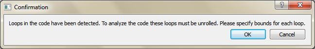
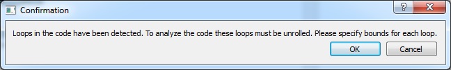
   This command should generate the test cases that correspond to the basis paths of the code in modexp_simple. A description of this command is provided in step 4 of tutorial 1. However, this time, GameTime ends its analysis with a notification that loops in the code have been detected. These loops need to be unrolled for any further analysis.

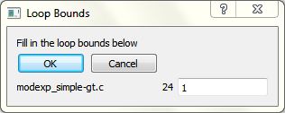
5. As per the instructions from GameTime, navigate to the temporary directory generated by GameTime for its analysis, located at sandbox/modexp/modexp_simple-gt. Examine the loop configuration file loop-config, and edit the third item of the first comma-separated line from 1 to 4.

   The loop configuration file informs the user of the locations of the loops within the file that is analyzed by GameTime, and allows the user to direct GameTime to unroll each loop a certain number of times.

   In the file, each line is a comma-separated list of three items: the name of the file that is analyzed by GameTime and contains loops (modexp_simple-gt.c), the line number of the header of the loop (24), and the number of times this loop should be unrolled (with a default value of 1).

   Note that, as declared in the loop configuration file, the file that is analyzed by GameTime is not the original file, but a copy of the file made by GameTime for the purposes of its analysis. This copy is stored within the temporary directory created by GameTime (modexp_simple-gt).

   Also note that, when the third item of the first line is edited from 1 to 4, the only loop in the code, whose header is at line 24, will be unrolled four times. This should result in code that is functionally equivalent to the code in tutorial 1, which performed modular exponentiation with four-bit exponents.

6. Run the following command at the prompt:

   analyze -a sandbox/modexp/projectConfig.xml --unroll-loops -b

   This command should generate the test cases that correspond to the basis paths of the code in modexp_simple, after its only loop has been unrolled.

   The command-line argument --unroll-loops instructs GameTime to unroll the loops in the code using the bounds provided by the user in the loop configuration file generated during loop detection.

7. If the previous step completes successfully, there should be another directory inside the project directory sandbox/modexp_simple besides the temporary directory modexp_simple-gt:

   The directory called analysis contains the results of the GameTime analysis that was just performed. The subdirectory basis stores all of the information regarding the basis paths of the code in modexp_simple (after its loop has been unrolled). In particular, the subdirectory case contains the test cases that correspond to the (five) basis paths of the code in modexp_simple (after its loop has been unrolled): the file labeled case-n contains the test case that corresponds to the nth basis path.

   Each of these test cases should be an assignment to the global variables in modexp_simple. For this tutorial, as in step 5 of tutorial 1, each test case assigns a value to the global variable exponent. Each test case will drive the execution of the function along a basis path.

8. Now that GameTime has generated the basis paths of the code in modexp_simple (after its loop has been unrolled) and the corresponding test cases, you can measure these test cases on the platform of your choice. For this tutorial, however, you can use the timing measurements already collected on the PTARM simulator, as stored in the directory simulations/ptarmsim-1.0.

   The file z3-glpk contains the timing measurements for the basis paths obtained in this tutorial. As the name of the file indicates, these measurements were made for the basis paths generated with Z3 as the SMT solver and GLPK as the ILP solver. (If you changed the SMT solver to Boolector in the project configuration file, you can use the file boolector-glpk for the next step instead.) These files are further described in step 6 of tutorial 1.

9. Run the following command in the root directory of the GameTime distribution:

   analyze -a sandbox/modexp/projectConfig.xml -d \
--values sandbox/modexp/simulations/ptarmsim-1.0/z3-glpk

   This command will generate the test cases that correspond to all (sixteen) of the feasible paths of the code in modexp_simple (after its loop has been unrolled).

   The command-line argument -d instructs the script to generate the test cases that correspond to all of the feasible paths of the code that is being analyzed, in decreasing order of their predicted timings. The other command-line arguments are further described in step 7 of tutorial 1.

10. If the previous step completes successfully, the directory called analysis, inside the project directory sandbox/modexp_simple, should now contain another subdirectory called all-dec.

    As with the subdirectory basis from step 7, the subdirectory all-dec also contains the subdirectory case, which stores the test cases that correspond to all of the (sixteen) feasible paths of the code in modexp-simple: the files are arranged in decreasing order of predicted timings, with the file labeled case-1 storing the test case for the (predicted) worst-case feasible path, and the file labeled case-16 storing the test case for the (predicted) best-case feasible path.

    Notice that the test case for the predicted worst-case feasible path assigns a value of 0xf to the global variable exponent. All of the four bits of exponent are thus set to 1. This indicates that the worst-case feasible path occurs when all four conditional statements in the code of modexp_simple evaluate to true. Also notice that the test case for the predicted best-case feasible path assigns a value of 0x0 to the global variable exponent, which implies that all four conditional statements evaluate to false.

    The predicted timings themselves are stored in the file labeled predicted-all-dec inside analysis. Each line has the number of a feasible path and the predicted timing of the corresponding test case, with the values separated by whitespace.

Tutorial 4: Overcomplete Basis

In this tutorial, we explore how to obtain more accurate estimates on the length of the longest path by generating (and measuring) more basis paths than the minimum number necessary. (As described in this paper). We will analyze a sample implementation of the insertion-sort algorithm sorting an array of a fixed size.

We begin by doing the same kind of analysis as in the previous tutorial. Then we explore how to generate and use larger sets of basis paths to obtain better and more accurate predictions of the longest paths. Finally, we compare the results obtained by both methods.

Setup

1. Run the executable gametime-cli located in the root directory of the GameTime distribution. This launches a command-line interface to GameTime: a window that contains a Cygwin prompt. Navigate to the root directory of the GameTime distribution.

2. Copy the directory labeled insertion_sort, which constitutes the GameTime project for this tutorial, from the demo/sandbox directory to the sandbox directory: cp -r demo/sandbox/insertion_sort sandbox

3. Examine the contents of the copied directory

   • The C file, insertion_sort.c, contains an implementation of the insertion-sort algorithm which sorts the global array of integers: a. We will analyze the code in the function insertion_sort. The constant LENGTH specifies the size of the array a. To keep the generated intermediate results small and the analysis fast, we use LENGTH = 8 in the tutorial.

   • The project configuration file, projectConfig.xml. Step 3 of tutorial 1 describes some of the tags in this file, and the documentation presents a comprehensive guide to all of these tags.

   • In this tutorial, we will introduce and describe a new parameter maximum-error-scale-factor in the projectConfig.xml file which directs GameTime to produce more accurate predictions.

   • In the tutorial, we will first run GameTime using the same approach as in the previous tutorials. Then we run GameTime with different algorithm for two different values of maximum-error-scale-factor. The subdirectory simulations/ptarmsim-1.0, contains timings of basis paths obtained using the PTARM simulator for the three cases: original-glpk-z3, error-10-glpk-z3, error-5-glpk-z3. (To install the PTARM simulator, please refer to step 3 of the installation guide. However, you do not need to install the simulator for this tutorial.)

4. The insertion-sort implementation analyzed in this tutorial contains two loops. As in the previous tutorial, we first unroll the loops up to the specified limit to obtain a loop-free code. Make sure you are in the root directory of the GameTime distribution and then run the following command at the prompt:

   analyze -a sandbox/insertion_sort/projectConfig.xml -b

   As in the previous tutorial, GameTime ends its analysis with a notification that loops in the code have been detected. These loops need to be unrolled for any further analysis.

5. As per the instructions from GameTime, navigate to the temporary directory generated by GameTime for its analysis, located at sandbox/insertion_sort/insertion_sort-gt. Examine the loop configuration file loop-config, and edit the third item of the first comma-separated line from 1 to 4 and the third item on the second comma-separated line from1 to 7

   For more details on the individual entries, see the description of the loop-config file in the previous tutorial. Note that the first line in the loop-config file corresponds to the inner while loop and the second line to the outer for loop in the insertion_sort function.

   Notice that we specify that the inner while loop in the insertion sort is unrolled only 4 times. In general, to always sort the input, the loop needs to be unrolled as many as 7 times. This intentional underspecification of the loop bound, yields a smaller program easier to analyse while still providing a relevant test cases and performance.

Timing Analysis

6. Now that we specified the desired unrolling, run the following command at the prompt:

   analyze -a sandbox/insertion_sort/projectConfig.xml --unroll-loops -b

   The command generates the test cases that correspond to the basis paths of the code in the function insertion_sort, after its loops have been unrolled (c.f., previous tutorial ) the specified number of times.

7. If the previous step completes successfully, another directory (analysis) should be created inside the project directory sandbox/insertion_sort (besides the temporary directory insertion_sort-gt).

   The directory analysis contains the results of the GameTime analysis that was just performed, see the previous tutorial for its description.

   For example, each generated test case, in directory sandbox/insertion_sort/analysis/basis/case is an assignment to the global array a that is then being sorted in the insertion_sort function. In total, 23 test cases should have been generated.

8. Now that GameTime has generated the basis paths of the code in insertion_sort (after its loops have been unrolled) and the corresponding test cases, you can measure these test cases on the platform of your choice. For this tutorial, however, you can use the timing measurements already collected on the PTARM simulator, as stored in the directory simulations/ptarmsim-1.0.

   The file original-glpk-z3 contains the timing measurements for the basis paths obtained in this tutorial for the basis paths generated in the previous steps. The file should contain 23 measurements; one for each basis path. Note that, in total, there is a total of 15000 paths in the control flow graph.

9. Run the following command in the root directory of the GameTime distribution:

   analyze -a sandbox/insertion_sort/projectConfig.xml -w -n 3 \
--values sandbox/insertion_sort/simulations/ptarmsim-1.0/original-glpk-z3

   This command will generate the test cases corresponding to the three feasible paths with the longest predicted length (specified by -w -n 3 flag) using the measurements from the given file.

   The projectConfig.xml file for the analyzed project has been configured to use Z3 SMT solver and the GLPK ILP solver. We provide measurements for the basis generated using these solvers.

10. If the previous step completes successfully, the directory called analysis, inside the project directory sandbox/insertion_sort, should now contain another subdirectory called worst.

    The subdirectory analysis/worst/case should now contain three files, the contents of which are the arguments corresponding to the three longest predicted paths. The predicted lengths of the paths can be found in the file analysis/predicted-worst. As of time of writing this tutorial, the predicted lengths are 6311, 6150, 6148 clock cycles respectively

    The lengths in the file predicted-worst are only the predictions for the paths corresponding to test cases in analysis/worst/case. Therefore, if we actually run the insertion_sort.c with the computed arguments, we expect, due to timing irregularities, the path lengths to differ.

    We have run the code in insertion-sort.c on the given test cases and measured the following lengths: 5766, 6045, 5605. As expected, the observed lengths differ from the predicted ones. Note that, due to timing irregularities, the path that corresponded to the second longest predicted path is actually longer than the one that was predicted to be the longest.

    If you have installed a simulator and specified the loop unrolling in the loop-config file, all values computed in this tutorial and the entire analysis until this point can be obtained by a single command:
    analyze -a sandbox/insertion_sort/projectConfig.xml -b -m -w -n -3 --unroll-loops
    If the above command terminates sucessfully and you have a simulator installed, GameTime creates a file analysis/measured-word containing the measured lengths of the three paths.

Timing Analysis using Overcomplete Basis

11. We now describe how to obtain more accurate predictions of paths lengths. This then allows us to find arguments on which insertion_sort runs longer than on any of the inputs computed in the previous steps.

    (Assumming the loops have been unrolled), run the following command in the gametime root directory (note that this overwrites the analysis from the previous steps): analyze -a sandbox/insertion_sort/projectConfig.xml -b --unroll-loops --overcomplete_basis

    The parameter --overcomplete_basis tells GameTime to generate more than the minimum number of basis paths necessary. The number of generated paths is determined by the desired accuracy of the algorithm as specified by the property maximum-error-scale-factor in sandbox/insertion_sort/projectConfig.xml. The parameter can be any real number of value at least 1. The lower the value, the more basis paths will be generated and more accurate the predicted lengths should be.

    Inspect the parameter maximum-error-scale-factor in sandbox/insertion_sort/projectConfig.xml file. Its value should be 10.0. In later steps we change this value and compare the accuracy of predictions.

    If the command runs successfully, GameTime should generate 27 basis paths (out of total number of 15000 paths in the underlying control-flow graph). This can be checked by inspecting the directory analysis/basis/case

12. To generate predictions using the overcomplete basis generated in the previous step, we need to use a dedicated algorithm that can make use of the additional basis paths. The algorithm is invoked by using the parameter --ob_extraction (standing for Overcomplete-Basis extraction).

    If you have not installed a simulator, we provide measurements of the basis paths on which the algorithm can be invoked. The measurements are in file sandbox/insertion_sort/simulations/ptarmsim-1.0/error-10-glpk-z3. You can use GameTime with the --ob_extraction flag by running:
    analyze -a sandbox/insertion_sort/projectConfig.xml -w -n 3 --ob_extraction \
--values sandbox/insertion_sort/simulations/ptarmsim-1.0/error-10-glpk-z3

    If you have a simulator installed, (if not, skip this step), you can obtain measurements and then the predictions directly by running the following command: analyze -a sandbox/insertion_sort/projectConfig.xml -m -w -n 3 --ob_extraction

    The flags --overcomplete_basis and --ob_extraction trigger new algorithms to compute the (overcomplete) basis and to predict the lengths of the longest path using this basis. (As described in this paper)

    While the flag --overcomplete_basis has to be used together with --ob_extraction, the opposite is not true. The flag --ob_extraction can be used without --ovecomplete_basis on the standard minimal basis generated by GameTime by default.

13. If the above command finished succesfully, there should be a file predicted-worst in the analysis directory with the lengths of the three longest predicted paths. The version of GameTime, as of writing this tutorial, generated the predictions: 6078, 6064, 6007. Note that these values are smaller than the ones in step 10.

    If you have a simulator installed, you can measure the actual path lengths for the corresponding inputs. In this case, the actual measured lengths turn out to be 5826, 6266, 5385. Note that not only are the measured values closer to the predicted values, they are also larger than the measured values in step 10 above.

    If the flag --ob_extraction is used, the accuracy of the predictions can be quantified more precisely. If the flag is used, GameTime produces two files mu-max and error-scale-factor in the analysis subdirectory. Both files contain a single number. It was shown that if the algorithm predicts (using the --ob_extraction flag) that the length of a path is L, then, under normal circumstances, the actual length of the path is within L +/- 2 * mu-max * error-scale-factor. In particular, to find the real longest paths, it suffices to generate paths until the difference in the length from the longest predicted path is more than 2 * mu-max * error-scale-factor.

    The parameter maximum-error-scale-factor in projectConfig.xml file tells GameTime to generate overcomplete basis so that the error-scale-factor is at most maximum-error-scale-factor.

    The value mu-max measures the timing irregularities in the program and the underlying platform; bigger values of mu-max correspond to bigger timing irregularities.

    It is important to stress that, unlike in the second part of this tutorial, using the --ob_extraction algorithm, GameTime is able to provide the error bounds on the generated predictions. In particular, the standard extraction procedure is unable to estimate the parameter mu-max measuring the timing irregularities in the underlying platform.

    If the command finished successfully, you should have mu-max = 74.18, error-scale-factor = 9.67 values. Using the formula in the box above, this yields an error bound of 2 * 74.18 * 9.67 = 1435

14. Now modify the value of maximum-error-scale-factor in sandbox/insertion_sort/projectConfig.xml file from 10.0 to 5.0. This tell GameTime to produce more accurate predictions and hence to generate larger overcomplete basis.

    Rerun the commands from the previous steps to generate an overcomplete basis and then use provided measurements (error-5-glpk-z3) to generate predictions using the following two commands:
    analyze -a sandbox/insertion_sort/projectConfig.xml -b --unroll-loops --overcomplete_basis
analyze -a sandbox/insertion_sort/projectConfig.xml -w -n 3 --ob_extraction \
--values sandbox/insertion_sort/simulations/ptarmsim-1.0/error-5-glpk-z3


    Note that the more accurate an estimate is required the longer the basis generation (first command) and the longest path predictions (second command) takes. On our machine (MacBook Air with 3.3GHz CPU), the first command took about 11 minutes to complete. If the above commands finish without any errors there should be a basis of size 48 and the lengths of the three predicted longest paths are: 6110, 6105, 6059.

    When measured, the actual lengths are 6288, 5603, 6427. Note that, not only the predictions are close to the measurements (mu-max = 128.60, error-scale-factor = 4.92, error_bound = 2 * 128.60 * 4.92 = 1265), but using a larger basis, we were able to generate longer paths than in any of the previous instances.

    Generating larger overcomplete basis yields, in general, better predictions. However, with better predictions comes bigger complexity. Be aware that as the basis gets bigger, the algorithm gets necessarily slower.

    In the extreme case of setting maximum-error-scale-factor to 1, one can prove that all feasbile paths need to be taken as the basis paths. Thus, GameTime exhaustively explores all paths in that case.

15. In this last step of the tutorial we analyse the results obtained in the three timing analyses perfomed in the tutorial. The insertion-sort algorithm sorts the array in the ascending order. Therefore, the "less sorted" the array is, the more steps the algorithm performs. Intuitively, we expecte the algorithm to takes the longest when the array ais sorted in descending order.

    The table below summarizes the paths found by GameTime in the three cases considered in this tutorial. In each of the three cases considered in this tutorial, we calculated three distinct paths. Each column in the table shows the values assigned to the array a which correspond to the path, out of the three predictions, that takes the longest when measured.

    Note that, the second column is far from sorted, whereas the last column is almost sorted except for a[5], a[6], a[7].

    A	Original	Maximum Error Scale Factor = 10	Maximum Error Scale Factor = 5
    a[0]	553648139	-2013265919	1083244544
    a[1]	1073741827	-2130444268	269486096
    a[2]	67117059	-2126512128	134217748
    a[3]	1066323	-2147483632	-2113929216
    a[4]	-2147483647	-2147483612	-2113929215
    a[5]	-2147483512	-2147483648	-2147483648
    a[6]	-2079326175	-2147483640	-2147475456
    a[7]	-214748364	-2147483648	-2147481534

Tutorial 1: Generating the Basis and Worst-Case Paths

In this tutorial, you will explore how to use the GUI to generate the test cases that correspond to the basis paths of exemplar code. You will then use pre-obtained measurements of these test cases to generate other test cases that correspond to the five worst-case paths (or the paths with the longest predicted timings).

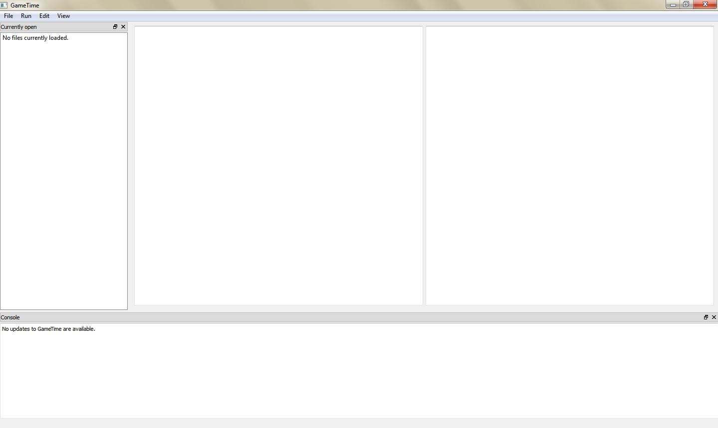
1. Run the executable gametime-gui located in the root directory of the GameTime distribution. This launches a GUI to GameTime. The interface has a main window and a background window that displays a verbose log of events. For this tutorial, you will be mostly concerned with the main window, shown below:

   

2. The GameTime distribution includes several sample projects within the demo/gui directory. Examine the contents of the subdirectory labeled modexp_unrolled, which constitutes the GameTime project for this tutorial:

   • The C file, modexp_simple.c, contains an implementation of modular exponentiation, where a base (the global variable base) is raised to an exponent (the global variable exponent), modulo a large prime number. The code that will be analyzed is present in a function called modexp_simple.

     The function implements the square-and-multiply algorithm, with one conditional statement for each bit of the exponent. Since there are only four conditional statements, this implementation is specific to four-bit exponents.

   • The directory simulations, which contains files that have the timings of the test cases that correspond to the basis paths of modexp_simple. The subdirectory ptarmsim-1.0 contains the timings as measured on the PTARM simulator. (To install the PTARM simulator, please refer to step 3 of the installation guide. However, you do not need to install the simulator for this tutorial.)

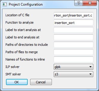
3. In the GameTime GUI, select File → Open project.... Navigate to the subdirectory demo/gui/modexp_unrolled and select the file modexp_simple.c. You may need to adjust the filter of the file picker to C files (*.c) to find and select the file. The following dialog box will pop up:

   

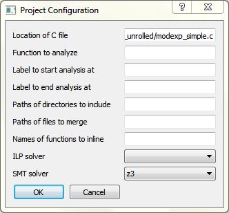
   The dialog box contains many fields that allow you to configure a GameTime project. In particular, the following fields are relevant for this tutorial:

   • Location of C file: The absolute location of the file that contains the code to be analyzed. This should be prepopulated with the absolute location of the file (modexp_simple.c) that was chosen in the file picker.

   • Function to analyze: The name of the function that is to be analyzed. Since the code in the function modexp_simple is to be analyzed, set this field to modexp_simple.

   • ILP solver: The name of the ILP solver that will be used by GameTime for its analysis. For this tutorial, set this field to glpk, which indicates that the ILP solver from GLPK will be used.

   • SMT solver: The name of the SMT solver that will be used by GameTime for its analysis. For this tutorial, set this field to z3, which indicates that Z3, the SMT solver from Microsoft, will be used. If you would like GameTime to use Boolector instead, set this to boolector (or any of the variants, whose suffixes are named after the SAT solver used by Boolector).

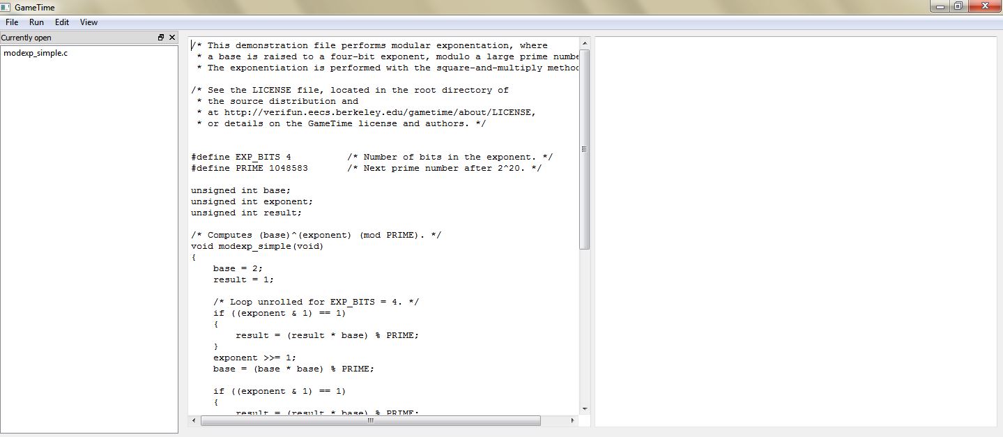
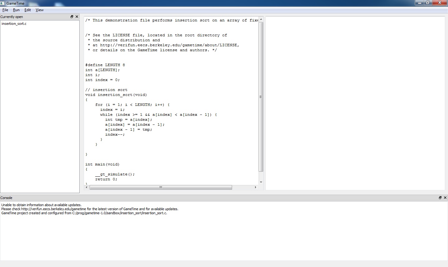
   Click OK. An entry for the file modexp_simple.c should be present in the leftmost window. Also, the code from the file should be loaded into the middle window, as shown below:

   

4. Select Run → Generate basis paths. This will generate the test cases that correspond to the basis paths of the code in modexp_simple. The Console, located in the bottom window, should display Generating basis paths.... Simultaneously, the background window displays a verbose log of events that occur as the basis paths are generated.

   Once done, the Console informs you that Basis paths have been generated. Also, the following dialog box will appear:

   

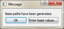
   Click OK to dismiss the dialog box.

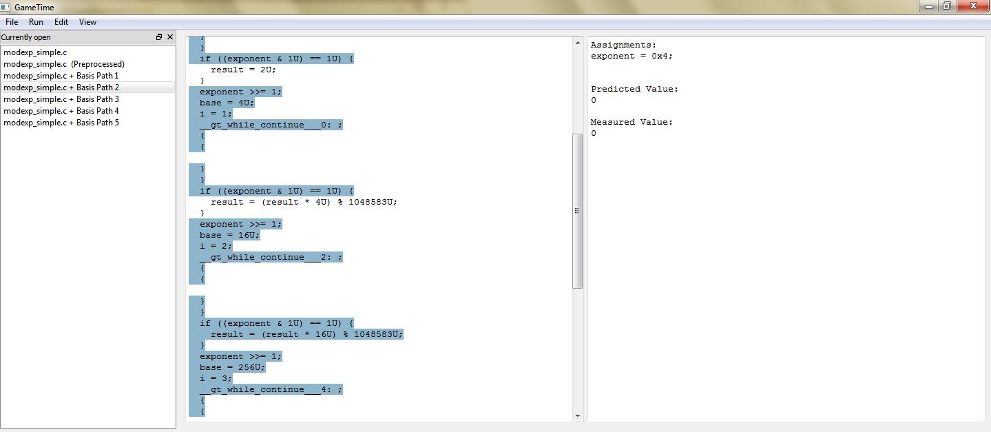
5. If the previous step completes successfully, the GUI should show new entries in the leftmost window, one for each of the newly generated basis paths. Double-click any one of these entries to highlight the statements executed along each path. For example, the image below shows the contents of the main window when you double-click the entry modexp_simple.c + Basis Path 2:

   

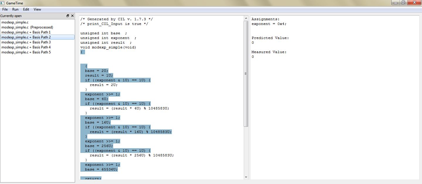
   The statements highlighted in the middle window represent the statements executed along the second basis path. The rightmost window shows the test case that corresponds to this basis path.

   Each test case that corresponds to each basis path is an assignment to the global variables in modexp_simple. For this tutorial, each test case assigns a value to the global variable exponent. Each test case will drive the execution of the function along a basis path.

   You may notice that the code displayed in the middle window is different from the original code. This is because GameTime uses CIL to preprocess the source code before analysis. You can examine this preprocessed code by double-clicking on the entry modexp_simple.c (Preprocessed).

6. Now that GameTime has generated the basis paths of the code in modexp_simple and the corresponding test cases, you can measure these test cases on the platform of your choice. For this tutorial, however, you can use the timing measurements already collected on the PTARM simulator, as stored in the directory simulations/ptarmsim-1.0.

   The file z3-glpk contains the timing measurements for the basis paths obtained in this tutorial. As the name of the file indicates, these measurements were made for the basis paths generated with Z3 as the SMT solver and GLPK as the ILP solver. (If you changed the SMT solver to Boolector in step 3, you can use the file boolector-glpk for this step instead.)

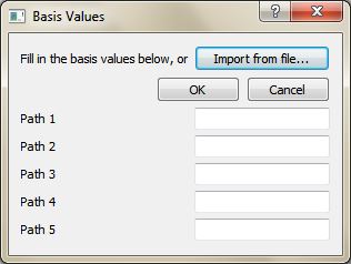
   In the file, lines that begin with the # character are comments. Each of the other lines in the file has the number of a basis path and the measurement of the corresponding test case on the PTARM simulator, with the values separated by whitespace.

   Select Edit → Enter basis values.... The following dialog box will appear:

   

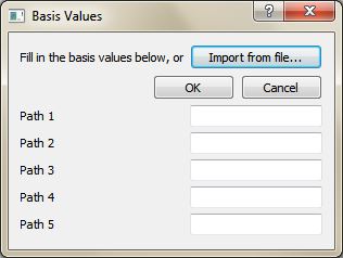
   Click Import from file... and, using the file picker that appears, select the appropriate file that contains the timing measurements for the basis paths (either simulations/ptarmsim-1.0/z3-glpk or simulations/ptarmsim-1.0/boolector-glpk). The dialog box should now populate with these measurements. Click OK.

7. Select Run → Generate worst-case feasible paths. In the dialog box that appears, enter 5:

   

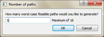
   This will generate the test cases that correspond to the five worst-case feasible paths of the code in modexp_simple. The Console, located in the bottom window, should display Generating 5 worst-case feasible paths.... Simultaneously, the background window displays a verbose log of events that occur as the worst-case feasible paths are generated.

   Once done, the Console informs you that 5 worst-case feasible paths have been generated. Also, the following dialog box will appear:

   

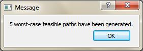
   Click OK to dismiss the dialog box.

8. If the previous step completes successfully, the GUI should show new entries in the leftmost window, one for each of the newly generated worst-case feasible paths. Double-click any one of these entries to highlight the statements executed along each path. For example, the image below shows the contents of the main window when you double-click the entry modexp_simple.c + Worst Path 1:

   

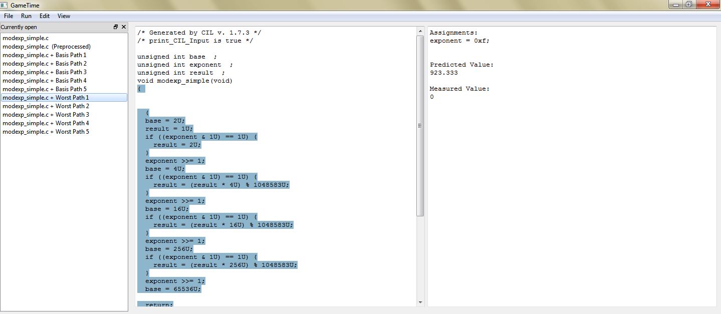
   The statements highlighted in the middle window represent the statements executed along the worst-case feasible path. The rightmost window shows the test case that corresponds to this path, and the predicted timing of this path.

   Notice that the test case for the predicted worst-case feasible path assigns a value of 0xf to the global variable exponent. All of the four bits of exponent are thus set to 1. This indicates that the worst-case feasible path occurs when all four conditional statements in the code of modexp_simple evaluate to true. In the test cases for the other four predicted worst-case feasible paths, exactly one bit of exponent is 0, which implies that exactly one of the four conditional statements evaluates to false.

Tutorial 2: Inlining Functions

In this tutorial, as in the previous tutorial, you will explore how to use the GUI to generate the test cases that correspond to the basis paths of exemplar code. However, this exemplar code calls another function, which thus needs to be inlined for the GameTime analysis. You will then use pre-obtained measurements of these test cases to generate other test cases that correspond to the five best-case paths (or the paths with the shortest predicted timings).

1. Run the executable gametime-gui located in the root directory of the GameTime distribution. This launches a GUI to GameTime. The interface has a main window and a background window that displays a verbose log of events. For this tutorial, you will be mostly concerned with the main window.

2. Within the demo/gui directory, examine the contents of the subdirectory labeled speed, which constitutes the GameTime project for this tutorial:

   • The C file, speed.c, contains code that calculates the final (one-dimensional) speed of an object with an initial speed (the global variable initial_speed) and constant acceleration (the global variable acc), after a certain amount of time (the global variable time). However, the final speed cannot exceed a certain predefined limit (the constant LIMIT, which here is assigned to 100). The code that will be analyzed is present in a function called calculate_final_speed. To ensure that the final speed does not exceed the limit, the function saturate is used: this is the function that needs to be inlined.

   • The directory simulations, which contains files that have the timings of the test cases that correspond to the basis paths of calculate_final_speed, after the function saturate has been inlined. The subdirectory ptarmsim-1.0 contains the timings as measured on the PTARM simulator. (To install the PTARM simulator, please refer to step 3 of the installation guide. However, you do not need to install the simulator for this tutorial.)

3. In the GameTime GUI, select File → Open project.... Navigate to the subdirectory demo/gui/speed and select the file speed.c. You may need to adjust the filter of the file picker to C files (*.c) to find and select the file. The following dialog box will pop up:

   

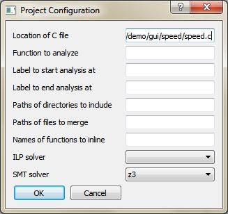
   The dialog box contains many fields that allow you to configure a GameTime project. In particular, the following fields are relevant for this tutorial:

   • Location of C file: The absolute location of the file that contains the code to be analyzed. This should be prepopulated with the absolute location of the file (speed.c) that was chosen in the file picker.

   • Function to analyze: The name of the function that is to be analyzed. Since the code in the function calculate_final_speed is to be analyzed, set this field to calculate_final_spped.

   • Names of functions to inline: The names of the functions that need to be inlined. The value of this field should be saturate, which is the name of the function that needs to be inlined into the function that is to be analyzed: calculate_final_speed.

   • ILP solver: The name of the ILP solver that will be used by GameTime for its analysis. For this tutorial, set this field to glpk, which indicates that the ILP solver from GLPK will be used.

   • SMT solver: The name of the SMT solver that will be used by GameTime for its analysis. For this tutorial, set this field to z3, which indicates that Z3, the SMT solver from Microsoft, will be used. If you would like GameTime to use Boolector instead, set this to boolector (or any of the variants, whose suffixes are named after the SAT solver used by Boolector).

   Click OK. An entry for the file speed.c should be present in the leftmost window. Also, the code from the file should be loaded into the middle window, as shown below:

   

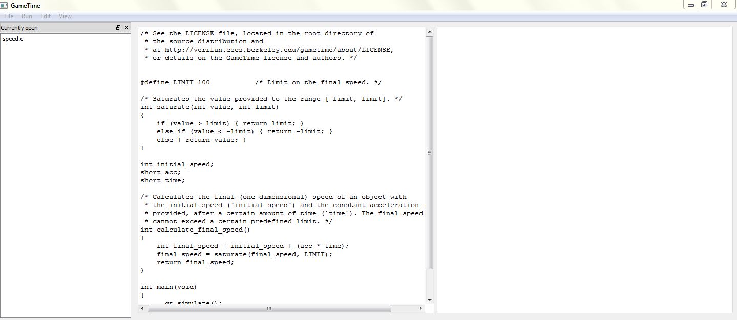
4. Select Run → Generate basis paths. This will generate the test cases that correspond to the basis paths of the code in calculate_final_speed, after inlining the function saturate. The Console, located in the bottom window, should display Generating basis paths.... Simultaneously, the background window displays a verbose log of events that occur as the basis paths are generated.

   Once done, the Console informs you that Basis paths have been generated. Also, the following dialog box will appear:

   

   Click OK to dismiss the dialog box.

5. If the previous step completes successfully, the GUI should show new entries in the leftmost window, one for each of the newly generated basis paths. Double-click any one of these entries to highlight the statements executed along each path. For example, the image below shows the contents of the main window when you double-click the entry speed.c + Basis Path 2:

   

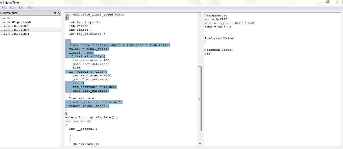
   The statements highlighted in the middle window represent the statements executed along the second basis path. The rightmost window shows the test case that corresponds to this basis path.

   Each test case that corresponds to each basis path is an assignment to the global variables in calculate_final_speed. Each test case will drive the execution of the function along a basis path.

   You may notice that the code displayed in the middle window is different from the original code. This is because GameTime uses CIL to preprocess the source code before analysis. You can examine this preprocessed code by double-clicking on the entry speed.c (Preprocessed): the middle window shows the code of the function calculate_final_speed, with the code in the function saturate inlined.

6. Now that GameTime has generated the basis paths of the code in calculate_final_speed (with the code in saturate inlined) and the corresponding test cases, you can measure these test cases on the platform of your choice. For this tutorial, however, you can use the timing measurements already collected on the PTARM simulator, as stored in the directory simulations/ptarmsim-1.0.

   The file z3-glpk contains the timing measurements for the basis paths obtained in this tutorial. As the name of the file indicates, these measurements were made for the basis paths generated with Z3 as the SMT solver and GLPK as the ILP solver. (If you changed the SMT solver to Boolector in step 3, you can use the file boolector-glpk for this step instead.) These files are further described in step 6 of tutorial 1.

   Select Edit → Enter basis values.... The following dialog box will appear:

   

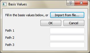
   Click Import from file... and, using the file picker that appears, select the appropriate file that contains the timing measurements for the basis paths (either simulations/ptarmsim-1.0/z3-glpk or simulations/ptarmsim-1.0/boolector-glpk). The dialog box should now populate with these measurements. Click OK.

7. Select Run → Generate best-case feasible paths. In the dialog box that appears, enter 3:

   

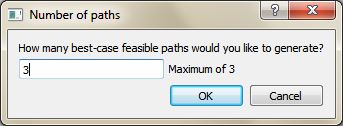
   This will generate the test cases that correspond to the three best-case feasible paths of the code in calculate_final_speed (with the code in saturate inlined). The Console, located in the bottom window, should display Generating 3 best-case feasible paths.... Simultaneously, the background window displays a verbose log of events that occur as the best-case feasible paths are generated.

   Once done, the Console informs you that 3 best-case feasible paths have been generated. Also, the following dialog box will appear:

   

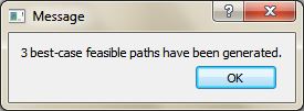
   Click OK to dismiss the dialog box.

8. If the previous step completes successfully, the GUI should show new entries in the leftmost window, one for each of the newly generated best-case feasible paths. Double-click any one of these entries to highlight the statements executed along each path. For example, the image below shows the contents of the main window when you double-click the entry speed.c + Best Path 1:

   

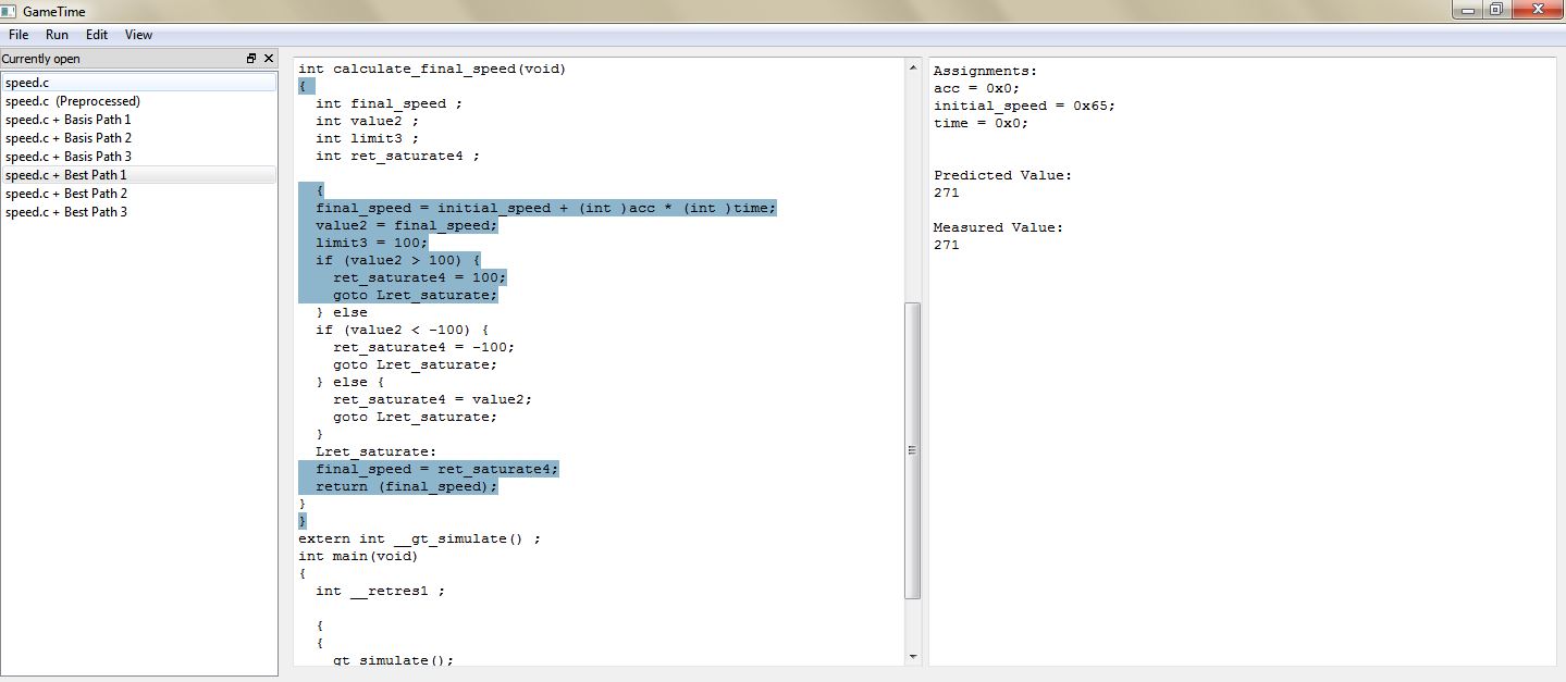
   The statements highlighted in the middle window represent the statements executed along the best-case feasible path. The rightmost window shows the test case that corresponds to this path, and the predicted timing of this path.

   Notice that the test case for the predicted best-case feasible path sets both the acceleration (acc) and the time (time) to zero, and sets the initial speed (initial_speed) to 0x65. These values produce a final speed (0x65) that satisfies the first condition of the only if-statement in the function saturate: value > LIMIT, where LIMIT is 100 (or 0x64).

   The test case for the next feasible path sets the global variables to values that produce a final speed. This speed does not satisfy the first condition of the if-statement, but satisfies the second condition. The execution of this feasible path thus needs two conditions to be evaluated, which results in a slightly longer timing for the path. Similarly, the execution of the third feasible path results in the evaluation of all three conditions, which results in the longest timing among the three predicted best-case feasible paths.

   The three feasible paths produced also correspond to the only three feasible paths through the function calculate_final_speed, after the function saturate has been inlined.

Tutorial 3: Unrolling Loops

In this tutorial, as in the previous two, you will explore how to use the GUI to generate the test cases that correspond to the basis paths of exemplar code. This code performs modular exponentiation, as the exemplar code from tutorial 1 does, but employs a for-loop to loop through the bits of the exponent. This loop needs to be unrolled for the GameTime analysis. You will then use pre-obtained measurements of the generated test cases to generate the test cases that correspond to all of the feasible paths.

1. Run the executable gametime-gui located in the root directory of the GameTime distribution. This launches a GUI to GameTime. The interface has a main window and a background window that displays a verbose log of events. For this tutorial, you will be mostly concerned with the main window.

2. Within the demo/gui directory, examine the contents of the subdirectory labeled modexp, which constitutes the GameTime project for this tutorial, and which should be similar to those in tutorial 1:

   • The C file, modexp_simple.c, contains an implementation of modular exponentiation, where a base (the global variable base) is raised to an exponent (the global variable exponent), modulo a large prime number. The code that will be analyzed is present in a function called modexp_simple. Notice that, unlike the code in tutorial 1, this implementation uses a for-loop.

   • The directory simulations, which contains files that have the timings of the test cases that correspond to the basis paths of calculate_final_speed, after the function saturate has been inlined. The subdirectory ptarmsim-1.0 contains the timings as measured on the PTARM simulator. (To install the PTARM simulator, please refer to step 3 of the installation guide. However, you do not need to install the simulator for this tutorial.)

3. In the GameTime GUI, select File → Open project.... Navigate to the subdirectory demo/gui/modexp and select the file modexp_simple.c. You may need to adjust the filter of the file picker to C files (*.c) to find and select the file. The following dialog box will pop up:

   

   The dialog box contains many fields that allow you to configure a GameTime project. In particular, the following fields are relevant for this tutorial:

   • Location of C file: The absolute location of the file that contains the code to be analyzed. This should be prepopulated with the absolute location of the file (modexp.c) that was chosen in the file picker.

   • Function to analyze: The name of the function that is to be analyzed. Since the code in the function modexp_simple is to be analyzed, set this field to modexp_simple.

   • ILP solver: The name of the ILP solver that will be used by GameTime for its analysis. For this tutorial, set this field to glpk, which indicates that the ILP solver from GLPK will be used.

   • SMT solver: The name of the SMT solver that will be used by GameTime for its analysis. For this tutorial, set this field to z3, which indicates that Z3, the SMT solver from Microsoft, will be used. If you would like GameTime to use Boolector instead, set this to boolector (or any of the variants, whose suffixes are named after the SAT solver used by Boolector).

   Click OK. An entry for the file modexp.c should be present in the leftmost window. Also, the code from the file should be loaded into the middle window, as shown below:

   

4. Select Run → Generate basis paths. As in step 4 of tutorial 1, this will generate the test cases that correspond to the basis paths of the code in modexp_simple. The Console, located in the bottom window, should display Generating basis paths.... Simultaneously, the background window displays a verbose log of events that occur as the basis paths are generated.

   However, this time, GameTime ends its analysis with a notification that the loops in the code have been detected:

   

   Click OK. Another dialog box will appear:

   

   Replace 1 with 4 and click OK.

   The dialog box informs the user of the locations of the loops within the file that is analyzed by GameTime, and allows the user to direct GameTime to unroll each loop a certain number of times.

   In the dialog box, each line contains three items: the name of the file that is analyzed by GameTime and contains loops (modexp_simple-gt.c), the line number of the header of the loop (24), and the number of times this loop should be unrolled (with a default value of 1).

   Note that, as seen in the dialog box, the file that is analyzed by GameTime is not the original file, but a copy of the file made by GameTime for the purposes of its analysis. This copy is stored within the temporary directory created by GameTime (modexp_simple-gt) in the same directory as the file that contains the code being analyzed.

   Also note that, when the third item of the first line is edited from 1 to 4, the only loop in the code, whose header is at line 24, will be unrolled four times. This should result in code that is functionally equivalent to the code in tutorial 1, which performed modular exponentiation with four-bit exponents.

   Once done, the Console informs you that Basis paths have been generated. Also, the following dialog box will appear:

   

   Click OK to dismiss the dialog box.

5. If the previous step completes successfully, the GUI should show new entries in the leftmost window, one for each of the newly generated basis paths. Double-click any one of these entries to highlight the statements executed along each path. For example, the image below shows the contents of the main window when you double-click the entry modexp.c + Basis Path 2:

   

   The statements highlighted in the middle window represent the statements executed along the second basis path. The rightmost window shows the test case that corresponds to this basis path.

   Each test case that corresponds to each basis path is an assignment to the global variables in modexp_simple. For this tutorial, as in step 5 of tutorial 1, each test case assigns a value to the global variable exponent. Each test case will drive the execution of the function along a basis path.

   You may notice that the code displayed in the middle window is different from the original code. This is because GameTime uses CIL to preprocess the source code before analysis. You can examine this preprocessed code by double-clicking on the entry modexp_simple.c (Preprocessed): the middle window shows the code of the function modexp_simple, with the only loop in the function unrolled four times.

6. Now that GameTime has generated the basis paths of the code in modexp_simple (after its loop has been unrolled) and the corresponding test cases, you can measure these test cases on the platform of your choice. For this tutorial, however, you can use the timing measurements already collected on the PTARM simulator, as stored in the directory simulations/ptarmsim-1.0.

   The file z3-glpk contains the timing measurements for the basis paths obtained in this tutorial. As the name of the file indicates, these measurements were made for the basis paths generated with Z3 as the SMT solver and GLPK as the ILP solver. (If you changed the SMT solver to Boolector in step 3, you can use the file boolector-glpk for this step instead.) These files are further described in step 6 of tutorial 1.

   Select Edit → Enter basis values.... The following dialog box will appear:

   

   Click Import from file... and, using the file picker that appears, select the appropriate file that contains the timing measurements for the basis paths (either simulations/ptarmsim-1.0/z3-glpk or simulations/ptarmsim-1.0/boolector-glpk). The dialog box should now populate with these measurements. Click OK.

7. Select Run → Generate all feasible paths (decreasing order). Click OK to dismiss the resulting warning:

   

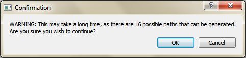
   This will generate the test cases that correspond to all (sixteen) of the feasible paths of the code in modexp_simple (after its loop has been unrolled), in decreasing order of their predicted timings. The Console, located in the bottom window, should display Generating all feasible paths in decreasing order of value.... Simultaneously, the background window displays a verbose log of events that occur as the best-case feasible paths are generated.

   Once done, the Console informs you that All feasible paths have been generated in decreasing order of value. Also, the following dialog box will appear:

   

   Click OK to dismiss the dialog box.

8. If the previous step completes successfully, the GUI should show new entries in the leftmost window, one for each of the newly generated feasible paths, arranged in decreasing order of predicted timings: the first feasible path is the (predicted) worst-case feasible path, while the last feasible path is the (predicted) best-case feasible path.

   Double-click any one of these entries to highlight the statements executed along each path. For example, the image below shows the contents of the main window when you double-click the entry modexp_simple.c + Path 1:

   

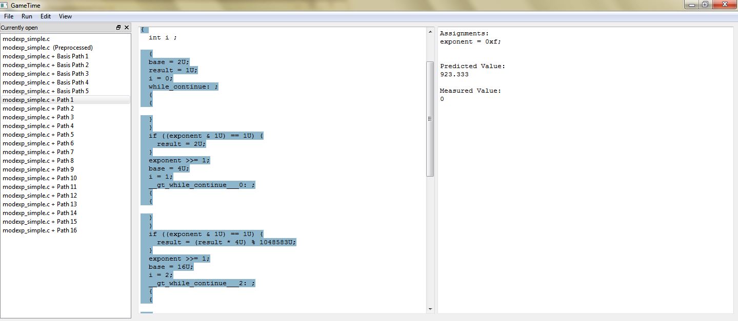
   The statements highlighted in the middle window represent the statements executed along the worst-case feasible path. The rightmost window shows the test case that corresponds to this path, and the predicted timing of this path.

   Notice that the test case for the predicted worst-case feasible path assigns a value of 0xf to the global variable exponent. All of the four bits of exponent are thus set to 1. This indicates that the worst-case feasible path occurs when all four conditional statements in the code of modexp_simple evaluate to true. Also notice that the test case for the predicted best-case feasible path assigns a value of 0x0 to the global variable exponent, which implies that all four conditional statements evaluate to false.

Tutorial 4: Overcomplete Basis

In this tutorial, we explore how to use GameTime GUI to obtain more accurate estimates on the length of the longest path by generating (and measuring) more basis paths than the minimum number necessary (as described in this paper). We will analyze a sample implementation of the insertion-sort algorithm sorting an array of a fixed size.

1. Run the executable gametime-gui located in the root directory of the GameTime distribution. This launches a GUI to GameTime. The interface has a main window and a background window that displays a verbose log of events. For this tutorial, you will be mostly concerned with the main window.

2. Within the demo/gui directory, examine the contents of the subdirectory labeled insertion_sort, which constitutes the GameTime project for this tutorial:

   • The C file, insertion_sort.c, contains an implementation of the insertion-sort algorithm which sorts the global array of integers: a. We will analyze the code in the function insertion_sort. The constant LENGTH specifies the size of the array a. To keep the generated intermediate results small and the analysis fast, we use LENGTH = 8 in the tutorial.

   • In the tutorial, we will first run GameTime using the same approach as in the previous tutorials. Then we run GameTime with different algorithm for two different values of Maximum Error Scale Factor. The subdirectory simulations/ptarmsim-1.0, contains timings of basis paths obtained using the PTARM simulator for the three cases: original-glpk-z3, error-10-glpk-z3, error-5-glpk-z3. (To install the PTARM simulator, please refer to step 3 of the installation guide. However, you do not need to install the simulator for this tutorial.)

3. In the GameTime GUI, select File → Open project.... Navigate to the subdirectory demo/gui/insertion_sort and select the file insertion_sort.c. You may need to adjust the filter of the file picker to C files (*.c) to find and select the file. A dialog appears. As described in the next paragraph, set the fields to the values shown in the picture:

   

   Specifically, the dialog box contains many fields that allow you to configure a GameTime project. The following fields are relevant for this tutorial:

   • Location of C file: The absolute location of the file that contains the code to be analyzed. This should be prepopulated with the absolute location of the file (insertion_sort.c) that was chosen in the file picker.

   • Function to analyze: The name of the function that is to be analyzed. Since the code in the function insertion_sort.c is to be analyzed, set this field to insertion_sort.

   • ILP solver: The name of the ILP solver that will be used by GameTime for its analysis. For this tutorial, set this field to glpk, which indicates that the ILP solver from GLPK will be used.

   • SMT solver: The name of the SMT solver that will be used by GameTime for its analysis. For this tutorial, set this field to z3, which indicates that Z3, the SMT solver from Microsoft, will be used. If you would like GameTime to use Boolector instead, set this to boolector (or any of the variants, whose suffixes are named after the SAT solver used by Boolector).

   Click OK. An entry for the file insertion_sort.c should be present in the leftmost window. Also, the code from the file should be loaded into the middle window, as shown below:

   

4. Select Run → Generate basis paths and approve the dialog that appers.

   

   As in step 4 of tutorial 1, this will generate the test cases that correspond to the basis paths of the code in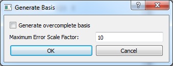 insertion_sort. The Console, located in the bottom window, should display Generating basis paths.... Simultaneously, the background window displays a verbose log of events that occur as the basis paths are generated.

   However, this time, GameTime ends its analysis with a notification that the loops in the code have been detected:

   

   Click OK. Another dialog box will appear, where we specify how many times the loops are unrolled. We proceed analogously to step 4, tutorial 3:

   

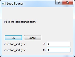
   Write 4 in the first field and 7 in the second field. Then click OK.

   The dialog box informs the user of the locations of the loops within the file that is analyzed by GameTime, and allows the user to direct GameTime to unroll each loop a certain number of times.

   The first line corresponds to the loop starting at line 20, which is the inner while loop. The second line specifies how many times the loop starting at line 18 should be unrolled. This corresponds to the outerfor loop in the insertion_sort function.

   Once done, the Console informs you that Basis paths have been generated. Also, the following dialog box will appear:

   

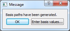
   Click OK to dismiss the dialog box.

5. If the previous step completes successfully, the GUI should show new entries in the leftmost window, one for each of the newly generated basis paths. There should be 23 paths in total. You can double-click any one of these entries to highlight the statements executed along each path.

   The statements highlighted in the middle window represent the statements executed along the basis path. The rightmost window shows the test case that corresponds to this basis path.

   Each test case that corresponds to each basis path is an assignment to the global variables in insertion_sort. Each test case will drive the execution of the function along a basis path.

   You may notice that the code displayed in the middle window is different from the original code. This is because GameTime uses CIL to preprocess the source code before analysis. You can examine this preprocessed code by double-clicking on the entry insertion_sort.c (Preprocessed): the middle window shows the code of the function insertion_sort, with the loops in the function unrolled accordingly to the values provided in the previous step.

6. Now that GameTime has generated the basis paths of the code in insertion_sort (after its loops have been unrolled) and the corresponding test cases, you can measure these test cases on the platform of your choice. For this tutorial, however, you can use the timing measurements already collected on the PTARM simulator, as stored in the directory simulations/ptarmsim-1.0.

   The file original-glpk-z3 contains the timing measurements for the 23 basis paths obtained in the previous steps. As the name of the file indicates, these measurements were made for the basis paths generated with Z3 as the SMT solver and GLPK as the ILP solver.

   Select Edit → Enter basis values.... The following dialog box will appear:

   

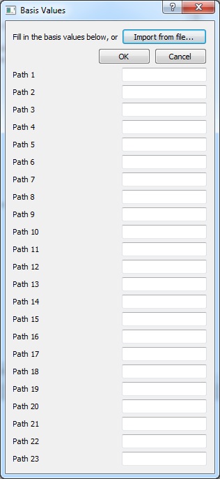
   Click Import from file... and, using the file picker that appears, select the appropriate file that contains the timing measurements for the basis paths: simulations/ptarmsim-1.0/original-glpk-z3

   

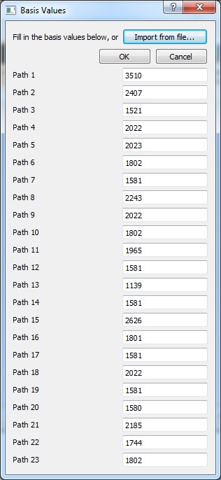
   The dialog box should now populate with these measurements. Click OK.

7. Select Run → Generate worst-case feasible paths. We want to generate three longest paths. Therefore, in the dialog that appears, write number 3 into the only editable text field. Click OK to proceed: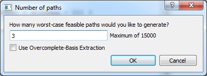

   

   This should generate test cases that correspond to three feasible paths in insertion_sort of the longest predicted length (in decreasing order of their predicted timings.) The Console, located in the bottom window, should display Generating 3 worst-case feasible paths.... Simultaneously, the background window displays a verbose log of events that occur as the paths are generated.

   Once done, the Console informs you that 3 worst-case feasible paths have been generated in decreasing order of value. Also, the following dialog box will appear:

   

   Click OK to dismiss the dialog box.

8. If the previous step completed successfully, the GUI should show three new entries in the leftmost window, one for each of the newly generated feasible paths, arranged in decreasing order of predicted timings: the first feasible path is the (predicted) worst-case feasible path, etc.

   Double-click any one of these entries to highlight the statements executed along each path.

   

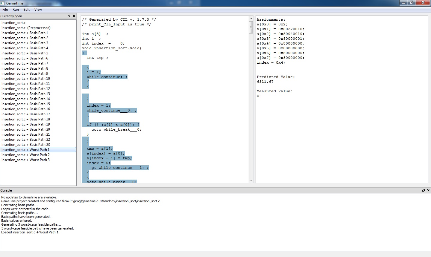
   The statements highlighted in the middle window represent the statements executed along the worst-case feasible path. The rightmost window shows the test case that corresponds to this path, and the predicted timing of this path. As of writing this tutorial, the predicted lengths of the three paths are 6311, 6150, 6148 clock cycles respectively.

   However, these are only predictions for the number clock cycles required to execute insertion_sort with the computed inputs. Therefore, if we actually run the insertion_sort.c with the computed arguments, we expect, due to timing irregularities, the path lengths to differ.

   We have run the code in insertion-sort.c on the given test cases and measured the following lengths: 5766, 6045, 5605. As expected, the observed lengths differ from the predicted ones. Note that, due to timing irregularities, the path that corresponded to the second longest predicted path is actually longer than the one that was predicted to be the longest.

   If you have installed a simulator, see step 10, tutorial 3 how all values computed in this tutorial and the entire analysis until this point can be obtained by a single command from the command line.

Timing Analysis using Overcomplete Basis

9. We now describe how to obtain more accurate predictions of paths lengths. This then allows us to find arguments on which insertion_sort runs longer than on any of the inputs computed in the previous steps.

   Run the Run → Generate basis paths command again. You will be notified that the basis paths generated in the previous steps will be deleted.

   

   Click OK to approve. On the next dialog , check the Generate overcomplete basis and in the text field below Maximum Error Scale Factor (which should now be editable), write 10. Then click OK.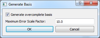

   

   The checkbox Generate overcomplete basis tells GameTime to generate more than the minimum number of basis paths necessary. The number of generated paths is determined by the desired accuracy of the algorithm as specified by the property Maximum Error Scale Factor. The parameter can be any real number of value at least 1. The lower the value, the more basis paths will be generated and more accurate the predicted lengths should be. (We use the value 10.0 in this step, but in later steps we will see the effect of using a different value.)

10. If the command runs successfully, GameTime should generate 27 basis paths (out of total number of 15000 paths in the underlying control-flow graph), which should appear in the leftmost column of the GUI

    As before, we provide measurements of the lengths of the basis paths as obtained by the Ptarmsim simulator. The measurements are loaded as in the previous steps: click on Edit → Enter basis values... and in the dialog click on Import from file option. Choose the file simulations/ptarmsim-1.0/error-10-glpk-z3.

    Once the file has been selected, the lengths of the basis paths are populated from the file. Click OK.

    

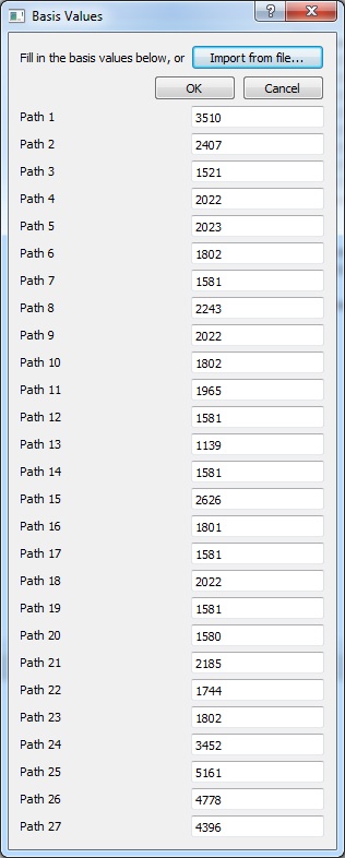
11. As in step 7 of this tutorial, we generate three longest paths. From the menu, select Run → Generate Worst-Case Feasible Paths.... A dialog appears and write 3 in the only field in the dialog to direct GameTime to find three paths.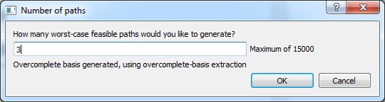

    

    Note the text under the only field in the dialog. It informs us that an overcomplate basis is being used and that GameTime is going to use a special algorithm that can make use of additional basis paths.

    Click OK and wait while GameTime generates predictions.

12. After a few moments a dialog informing us of the end of the analysis appears. If the command finished succesfully, three more paths should appear in the list in the leftmost column. You can inspect them by double clicking on them.

    With each path, GameTime provides a predicted length of the path. The version of GameTime as of writing this tutorial generated the predictions of lengths 6078, 6064, 6007, respectively. Note that these values are smaller than the ones in step 8.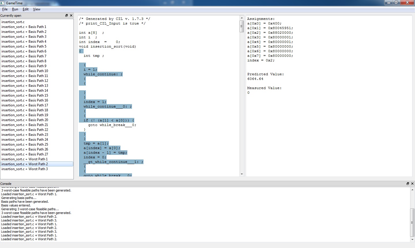

    

    If you have a simulator installed, you can measure the actual path lengths for the corresponding inputs. In this case, the actual measured lengths turn out to be 5826, 6266, 5385. Note that not only are the measured values closer to the predicted values, they are also larger than the measured values in step 8 above.

    Furthermore, if the predictions are generated using an overcomplete-basis extraction then it is possible to bound the difference between the predicted and measured path lengths, as described in the box in step 13 in the fourth command-line tutorial.

13. In the remaining steps, we tell GameTime to generate even more accurate predictions.

    As before, click on Run → Generate basis paths.... First confirm that you wish to delete all generated paths. Then in the dialog that appears, check Generate overcomplete basis and write 5.0 into the text field. Click OK.

14. Note that the more accurate an estimate is required the longer the basis generation takes. On our machine, the command took about 11 minutes to complete. You can check that GameTime is computing the basis by observing the background window where GameTime constantly outputs information about computation. If the computation finishes without any errors there should be a basis of size 48; the paths appearing in the leftmost column.

15. We provide measurements of the lengths of the basis paths in this situation as well. Load the measurement length of the basis paths: Click on Edit → Enter basis values, in the dialog import basis lengths from file simulations/ptarmsim-1.0/error-5-glpk-z3 and click OK.

16. Finally, we generate predictions. Click on Run → Generate worst-case feasible paths. In the text field write 3 specifying that we want GameTime to generate three predictions. Then click OK.

    Wait a few momements while GameTime generate predictions. If the command finishes sucessfully, the lengths of the three predicted longest paths should be: 6110, 6105, 6059.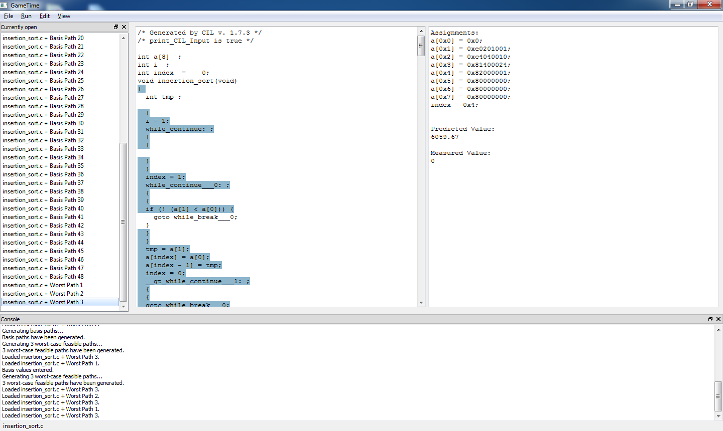

    

    When measured, the actual lengths are 6288, 5603, 6427. Note that, not only the predictions are close to the measurements but using a larger basis, we were able to generate longer paths than in any of the previous instances.

    Generating larger overcomplete basis yields, in general, better predictions. However, with better predictions comes bigger complexity. Be aware that as the basis gets bigger, the algorithm gets necessarily slower.

    In the extreme case of setting maximum-error-scale-factor to 1, one can prove that all feasbile paths need to be taken as the basis paths. Thus, GameTime exhaustively explores all paths in that case.